
More precisely, a sampling technique for situations where one of two correlated variables is easy to measure, while the other is not.
Say you wanted to correlate a personality questionnaire with a neural measure. Or a result from a behavioural experiment with a neural measure. This is not easy, because (a) when such correlations exist, they tend to be small, and (b) it takes too long and costs too much to collect a sufficient number of neuroimaging datasets. If the correlation in the population is 0.25, and you collected data from 70 randomly selected people, then your chance of finding a significant correlation is only about 50%. A coin flip.
The chance of finding a neuroimaging paper with 70 participants is quite a bit lower than a coin flip too, but it is not unfeasible. I thought I could do that, if I could find a way to boost power using non-random sampling. For my easy to measure measure, people need to spend 5-10 minutes at their computer filling a questionnaire. I can collect as many of these as I like. And then decide who to bring to the lab for the EEG. Is there a way to do this that would increase power?
It so happens that there is: oversample from the tails of the distribution.
I first generated a multivariate normal distribution with two variables (10K measures each) that correlate with a predefined value. Then I sampled from this population, either randomly (70 people), or heavily from the tails (30 each) and a little bit (10) from the middle:
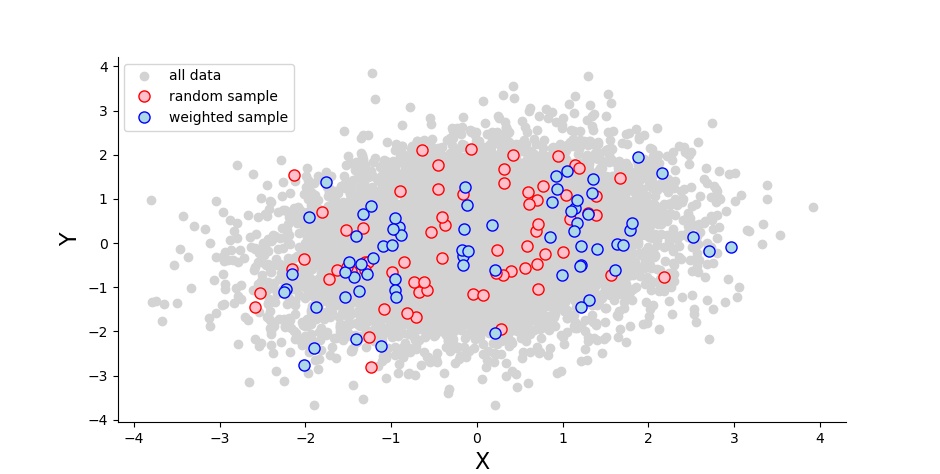
I ran a Pearson correlation for both the random sample (the blue dots) and the weighted sample (red). I did this 1000 times, and noted how often the p-values were significant as well as how high the correlation coefficients were. I ran this for a range of correlation coefficients spanning from 0 to 1. And I sent a description much like this one to my colleague Sam Parsons, who then based on it wrote his own code to do the same. (Scroll down for my python and his R code.)
And what did we both get? A veritable power boost for small true correlation values.
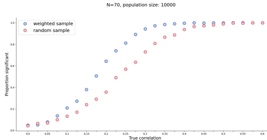
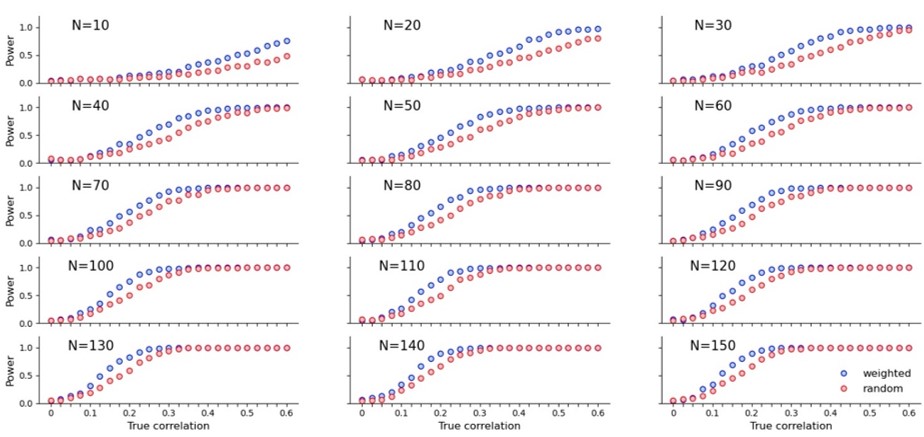
Initially I wondered whether this sampling method might create correlations out of noise, but when the true correlation is zero, a weighted sample finds a significant correlation as often as a random sample. The real power boost started around r=0.075 and stopped after r=0.45. With a sample of 70 people I only needed the true correlation to be 0.325 to reach power approaching 100%. With random sampling that correlation would need to be about 0.45. (For 80% power at N=70 that’s r=0.25 for weighted sampling vs. r=0.35 for random sampling.) So far so good.
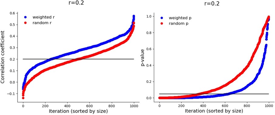
Are the correlation values that the method gives similar to the true correlation? Actually, no, they are not. The correlations are artificially inflated (or deflated, if lower than 0), which is probably how the significance values are boosted. Take a look at the different iterations in a population with a true correlation coefficient of 0.2:
But again – this inflation only happens when there is a true correlation. If it is zero:
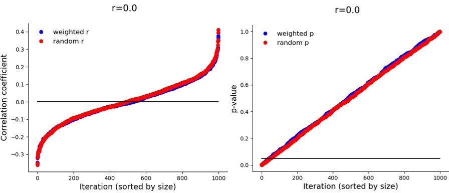
In the future I will try to see if simulations can be used to calculate an r_adjusted. In the absence of that, this sampling methods boosts power so that it increases the likelihood of finding a true correlation in a small sample, but its obtained correlation coefficient is likely to overestimate the true correlation. (Under the condition that (a) the measurement instrument accurately captures the entire range of the population distribution, which (b) is normal.)
Here is what the power boost looks like for a variety of sample sizes:
Is this sampling method used elsewhere? Yes. I vaguely remember seeing something similar in a blog post which I think was medical and I think employed ANOVA. I couldn’t track it down, nor could I find the exact word combination for Google to take me to the right statistical papers. I’m wondering if this type of sampling has a name, or if someone maybe knows which blog post I’m talking about.
I am also posting here because I’m interested in hearing opinions about the potential pitfalls of this approach, as well as figuring out under which conditions it shouldn’t be done. Should I use this approach in my next experiment? Is it a way to assess individual differences with smaller samples? Talk to me!
PS: Here’s the code. Python:
# import libraries
import numpy as np
import matplotlib.pyplot as plt
import scipy.stats as stats
import random

population=10000 # population size
total_iter = 1000 # iterations per population correlation

mean = [0, 0]
fignum = 0

power_rand, power_weight = list(), list()
xticks = list()

for true_corr in np.linspace(0,0.6,25): # iterate over correlation values
    true_corr = round(true_corr,3)
    print(true_corr)
    xticks.append(true_corr)

    cov = [[1.0, true_corr], [true_corr, 1.0]]
    iteration=0

    r_random, r_weighted = list(), list()
    p_random, p_weighted = list(), list()

    for iteration in range(total_iter): # sample many times from population
        g = random.Random()
        g.seed(random.randint(1,500))

    # create X and Y multivariate normal distribution

        x, y = np.random.multivariate_normal(mean, cov, population).T
        data = np.stack((np.array(x), np.array(y)), axis=-1)

    # sort X and Y variables by ascending X

        data = data[np.argsort(data[:, 0])]

       ### SELECT WEIGHTED SAMPLE ###

    # randomly select 30 from each tail and 10 from middle
        tail, middle = 30, 10
        sample_size = tail*2 + middle

        total_indices = len(data)
        border_index = int(len(data)/5)

        weighted_indices =[g.sample(range(border_index),tail) + g.sample(range(border_index*2, border_index*3),middle) + g.sample(range(border_index*4, border_index*5),tail)][0]
        data_weighted = data[weighted_indices,:]

    # collect into two variables, x_weighted_sample and y_weighted_sample

        x_weighted_sample = [item[0] for item in data_weighted]
        y_weighted_sample = [item[1] for item in data_weighted]

    # save correlation coefficient and significance value
        rho_weighted, p_val = stats.pearsonr(x_weighted_sample, y_weighted_sample)
        r_weighted.append(rho_weighted)
        p_weighted.append(p_val)

        ### SELECT RANDOM SAMPLE ###

        ind_random = g.sample(range(len(x)),sample_size)
        x_random_sample = list(x[ind_random])
        y_random_sample = list(y[ind_random])

        rho_random, p_val = stats.pearsonr(x_random_sample, y_random_sample)
        r_random.append(rho_random)
        p_random.append(p_val)


# prepare p values, correlations and power for plotting

    p_random = np.array(p_random)
    p_random = p_random[np.argsort(p_random)]
    p_weighted= np.array(p_weighted)
    p_weighted = p_weighted[np.argsort(p_weighted)]

    r_weighted = np.array(r_weighted)
    r_weighted = r_weighted[np.argsort(r_weighted)]
    r_random = np.array(r_random)
    r_random = r_random[np.argsort(r_random)]

    p_sig_random = p_random[p_random<0.05]
    power_random = len(p_sig_random) / total_iter
    p_sig_weighted = p_weighted[p_weighted<0.05]
    power_weighted= len(p_sig_weighted) / total_iter

    power_rand.append(power_random)
    power_weight.append(power_weighted)


'''
    # plot data
    fig, ax = plt.subplots()
    fignum+=1
    plt.plot(r_weighted, 'bo', label = 'weighted r')
    plt.plot(r_random, 'ro', label = 'random r')
    plt.legend(fontsize=12, frameon = False)
    x_coordinates = [0, iteration]
    y_coordinates = [true_corr, true_corr]
    plt.plot(x_coordinates, y_coordinates, 'k')
    plt.suptitle(f"r={true_corr}", fontsize=16)
    plt.xlabel('Iteration (sorted by size)', fontsize=14)
    plt.ylabel('Correlation coefficient', fontsize=14)

    right_side = ax.spines["right"]
    right_side.set_visible(False)
    upper_side = ax.spines["top"]
    upper_side.set_visible(False)

    plt.savefig(f'SimPlot{fignum}_WEIGHTED.jpg')

    fig, ax = plt.subplots()
    fignum+=1
    plt.plot(p_weighted, 'bo', label = 'weighted p')
    plt.plot(p_random, 'ro', label = 'random p')
    plt.legend(fontsize=12, frameon = False)
    y_coordinates = [0.05, 0.05]
    plt.plot(x_coordinates, y_coordinates, 'k')
    plt.suptitle(f"r={true_corr}", fontsize=16)
    plt.xlabel('Iteration (sorted by size)', fontsize=14)
    plt.ylabel('p-value', fontsize=14)

    right_side = ax.spines["right"]
    right_side.set_visible(False)
    upper_side = ax.spines["top"]
    upper_side.set_visible(False)

    plt.savefig(f'SimPlot{fignum}_WEIGHTED.jpg')
    plt.close('all')

#'''

# PLOT overall power

for i in range(len(xticks)):
    if i%2 != 0:
        xticks[i]= ''

fig, ax = plt.subplots(figsize=(18,8))
fignum+=1
plt.plot(power_weight, 'o', label = 'weighted sample', markerfacecolor='lightblue', markeredgecolor="blue", markersize = 11)
plt.plot(power_rand, 'o', label = 'random sample', markerfacecolor='pink', markeredgecolor="red", markersize = 11)
plt.legend(fontsize=18)#, frameon = False)
plt.xticks(np.arange(0, 25, step=1), xticks)
plt.xlabel('True correlation', fontsize=16)
plt.ylabel('Proportion significant', fontsize=16)
plt.suptitle(f'N={sample_size}, population size: {population}', fontsize=18)

right_side = ax.spines["right"]
right_side.set_visible(False)
upper_side = ax.spines["top"]
upper_side.set_visible(False)

plt.savefig(f'SimPlot{fignum}_WEIGHTED.jpg')

'''

fig, ax = plt.subplots(figsize=(18,8))
plt.plot(data[:,0], data[:,1], 'o', markerfacecolor='lightgrey', markeredgecolor="lightgrey", label = 'all data')
plt.plot(x_random_sample, y_random_sample, 'o', markerfacecolor='lightblue', markeredgecolor="blue", markersize = 11, label = 'random sample')
plt.plot(x_weighted_sample, y_weighted_sample, 'o', markerfacecolor='pink', markeredgecolor="red", markersize = 11, label = 'weighted sample')
plt.legend(fontsize=14)
right_side = ax.spines["right"]
right_side.set_visible(False)
upper_side = ax.spines["top"]
upper_side.set_visible(False)
plt.xlabel('X', fontsize=16)
plt.ylabel('Y', fontsize=16)


'''
And Sam’s R code:
# required packages
library("tidyverse")  #always
library('MASS') # to simulate correlated data

# to be edited
pop_size = 10000  # population to draw from
pop_cors = seq(.05, .95, .05) # population correlation
sims = 1000 # number of simulations to run
sample_size = 70 # sample size to extract


out_data <- data.frame(pop_cors = pop_cors,
                       power = NA,
                       power_weighted = NA,
                       mean_effect = NA,
                       mean_effect_weighted = NA)
count <- 1

for(r in pop_cors) {

# generate sigma matrix
sigma <- matrix(c(1, r,
                  r, 1),
                nrow=2)

# generate simulated data
pop_data = as.data.frame(
  mvrnorm(n = pop_size,
               mu = c(0, 0),
               Sigma = sigma, empirical = TRUE)
  )

sim_data <- data.frame(sim = 1:sims,
                       r = NA,
                       p = NA)


# unweighted
for(i in 1:sims) {

temp_data <- dplyr::sample_n(pop_data, sample_size)

temp_cor <- cor.test(temp_data[, 1],
                     temp_data[, 2])

sim_data[i,"r"] <- temp_cor$estimate
sim_data[i, "p"] <- temp_cor$p.value

}

#weighted quintiles 30,0,10,30
sim_data_weighted <- data.frame(sim = 1:sims,
                       r = NA,
                       p = NA)

for(i in 1:sims) {

pop_data2 <- pop_data
pop_data2$ntile <- ntile(pop_data2$V1, 5)
lower <- subset(pop_data2, ntile == 1)
mid <- subset(pop_data2, ntile == 3)
upper <- subset(pop_data2, ntile == 5)


weighted_sim <- rbind(
  sample_n(lower, 30),
  sample_n(mid, 10),
  sample_n(upper, 30)
)

temp_cor_weighted <- cor.test(weighted_sim[, 1],
                              weighted_sim[, 2])

sim_data_weighted[i,"r"] <- temp_cor_weighted$estimate
sim_data_weighted[i, "p"] <- temp_cor_weighted$p.value

}

###


out_data[count, "power"] <- sum(sim_data$p < .05) / sims

out_data[count, "mean_effect"] <- mean(sim_data$r)


out_data[count, "power_weighted"] <- sum(sim_data_weighted$p < .05) / sims

out_data[count, "mean_effect_weighted"] <- mean(sim_data_weighted$r)


count <- count + 1

}


#############################

closed_form <- pwr::pwr.r.test(n = sample_size,
                r = pop_cors)
closed_form2 <- data.frame(pop_cors = closed_form$r,
                           power2 = closed_form$power)

closed_form2 %>%
  as.data.frame() %>%
  ggplot(aes(x = pop_cors, y = power2)) +
  geom_point()


##############################
# some figures

together <- left_join(out_data, closed_form2, by = "pop_cors")

together %>%
  dplyr::select(pop_cors,
         power,
         power_weighted,
         power2) %>%
  gather(key = "sim",
         value = "power",
         -pop_cors) %>%
  ggplot(aes(x = pop_cors, y = power, colour = sim)) +
  geom_point() +
  geom_line()

together %>%
  dplyr::select(pop_cors,
                mean_effect,
                mean_effect_weighted) %>%
  gather(key = "sim",
         value = "effect",
         -pop_cors) %>%
  ggplot(aes(x = pop_cors, y = effect, colour = sim)) +
  geom_point() +
  geom_line()
To cite this blog post, please use: Todorovic, Ana. “A sampling technique for individual differences in neural data”. Web blog post. NeuroAnaTody.com, published May 2020. Web.