How many times have you read a research paper only to say, I don’t really believe this finding. It’s a regular occurrence, isn’t it? There is just something about the evidence that isn’t strong enough despite statistical significance, something about your theoretical knowledge that makes this finding fit rather badly. You perform a calculation in your mind, weighing the chance that it is false against the chance that it might be true, given what you already know.
Why not integrate that process (of comparing different outcomes to each other in light of previous knowledge) into your statistical test?
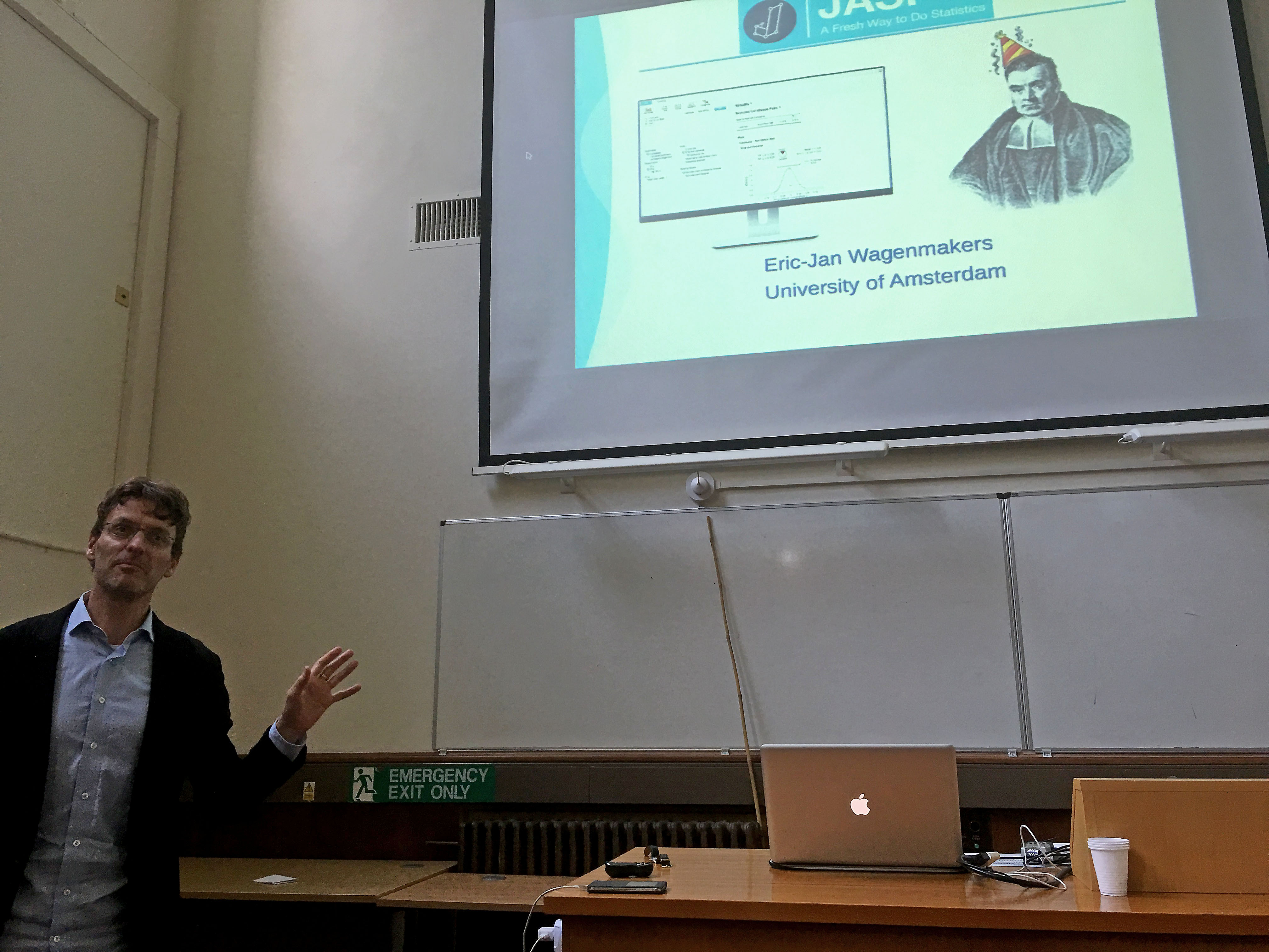
This is what EJ Wagenmakers talked about when he introduced us to Bayesian statistics without tears.
The Bayesian approach involves an epistemological shift regarding how statistics fit our research questions. EJ described several elements of what it means to go Bayesian, with a strong emphasis on how we can think about testing data and what we are allowed to conclude.
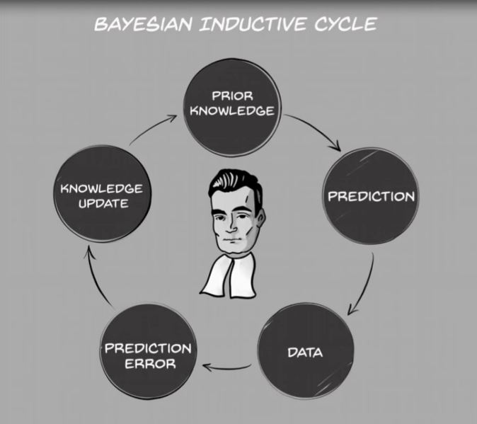
The Bayesian inductive cycle consists of the following. First, we go into empirical investigations with some background of previous findings, of prior knowledge. We form an educated guess – a prediction – based on this knowledge. We collect data. We quantify how wrong we were about our prediction, given the data. Then we update our knowledge, which leads to an update in our predictions, and the cycle begins anew. Note how different this is from the roundabout process of concluding there is evidence for our hypothesis if the null is unlikely, while at the same time not being able to determine whether the null is likely. (Did that last sentence even make sense? Exactly!)
A critical difference between Bayesian testing and frequentist statistics, is that hypotheses can be tested against each other. You might think one outcome is likely, someone else might think another outcome is likely – why not compare the two directly? A natural consequence of this approach is that we then also discuss outcomes in the context of theoretical models (this model is more accurate than that model), rather than as absolute truths (the null is unlikely therefore my model is right).
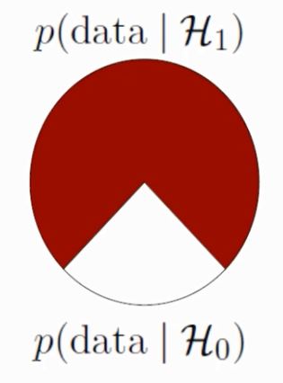
How do we quantify evidence for one hypothesis over the other? With the Bayes factor. A Bayes factor tells us how many times more the data align with one tested hypothesis than with the other. And this is not all – there’s pizza as well.
Pizza?
Yes, pizza. EJ described Bayes factors through so-called pizza plots. Suppose we have a Bayes factor of 3, for a test with 4 possible outcomes. Given that both hypotheses are equally likely a priori, this means the likelihood of our hypothesis being true is ¾, or 75%. Now let’s make some pizza. Cover 75% with pepperoni, and 25% with mozzarella. Very good. Now – no, don’t eat it yet – now put it on a spinning plate, close your eyes and dip a finger into the pizza. Your finger fell into the mozzarella part – how surprising do you find that? Probably not very surprising, which is why a Bayes factor of 3 is not considered particularly strong evidence. One hypothesis is likely, but the other hypothesis might well be true after all. And a p-value close to 0.05 corresponds to weaker evidence than a Bayes factor of 3…
Bayes methodology can also give evidence in favour of a null hypothesis (i.e. for the absence of an effect). This is especially important in replication studies.
Finally, EJ talked became about zombies. Are all zombies hungry? A little girl has observed 12 and they were all hungry, but what about other zombies? Take a look at the video to see how she deals with this question like a true Bayesian:
(This blog post is a preview of the themes in EJ Wagenmakers’ talk at the Oxford Reproducibility School, held on September 27, 2017. I occasionally use my own words to describe the contents, but the presented ideas do not deviate from the talk.)