
I read a few papers and wanted to share my thoughts with the cognitive science community. If phrases like predictive coding, mismatch negativity, or gamma band don’t mean much to you, the rest of the text is likely to be mind-numbingly boring.
Mismatch negativity
If we hear a train of identical tones, occasionally interrupted by a tone of a different pitch, the neural response to this new tone will be increased. The ERP difference wave between these frequent standards and infrequent deviants/oddballs, is called the mismatch negativity. The neural generators of this difference wave are typically found bilaterally in the temporal lobes, as well as in the right frontal cortex.
The size of the difference wave depends on probabilistic features of the stimulation, such as how often the oddball will be displayed, but also on physical features, such as how distant in pitch the standard and the oddball tones are.
The negativity in the name comes from the sign of the deflection of the electrical signal, and is not descriptive of the neural or the cognitive processing. Mismatch is a cognitive label, suggesting that the difference wave arises as a function of the difference between an internal memory trace and current input.
The description of this neural effect is intuitive but somewhat black-boxy, and is going out of fashion. The more physiologically informed framework of predictive coding is used to interpret it increasingly often.
Predictive coding
Predictive coding models rely on the idea that each functionally specific cortical area is dedicated to processing not only the type of information that it is geared to process (like line orientation in V1 or motion in MT), but also the statistical regularities present in that information (like the existence many parallel bars that form a fence, or the combined motion of a flock of geese).
The specifics of these regularities are passed back and forth between brain areas: the already extracted regularities are fed backwards through the cortical hierarchy, and this is visible in changes in alpha/beta synchronization, while the differences between the previous, ‘expected’ regularity and current input is fed forward to the next cortical area, and this is visible in gamma band power. So even if V1 couldn’t take into account the entire formation of the fence itself, back-projections from inferotemporal cortex will allow it to (also) respond to statistics present in the totality of the object.
Prediction errors arising from one area are used to fine-tune the neural representation of the statistics of the sensory input in the next cortical area, and these are again fed back, leading to an iterative adjustment of the next prediction.
The higher the discrepancy between the real and expected input, the greater the increase in net neural activity. Taken together, input that is statistically unlikely (based on previous input), should lead to (1) stronger neural activity, as evidenced by an increase in ERP/ERF/LFPs or BOLD response, (2) an increase in gamma power, (3) a decrease in alpha/beta power – or at least, findings of these types are interpreted to align with predictive coding… with many, many variations.
Predictive hypotheses?
The (somato)sensory brain certainly picks up statistical regularities with ease, but this doesn’t automatically mean the models are accurate. Their aim for generality on the one hand (they are supposed to unearth the common computational ground for all of cognition), and the post hoc confirmatory language of scientific writing on the other hand, makes it difficult to asses how fine-tuned hypotheses the models can deliver.
The models assume that similar information is being processed within larger and larger receptive fields as we go up the cortical hierarchy, with statistical properties concurrently being constrained with more and more precision. However, a number of aspects of information processing diverge from this. Colour processing, for example, appears to be largely redundant, processed over and over in a number of visual areas. Perception of time (very sensitive to statistical regularities) involves a large network of concerted activity rather than a set of areas that specifically break time down into smaller nuggets.
The models don’t make a clear prediction on whether an error should resolve within one brain area, two connected areas, or if we should see the traces of a prediction and error in the entire space of information processing, regardless of where it arose. Some of the theory does try to connect semantics to sensory processing (predictions all the way down), but the real models are more modest, and data align to this full-blown integration only rarely (but maybe errors reach all the way up).
Local and global mismatch negativity
Here I’ll put three mismatch negativity papers side by side (in order of appearance), and compare their findings in light of predictive coding.
All three involve two types of auditory predictability: local changes (from one tone pitch to another) and global structures (of repetitive series of five tones).
For example, if a train of 5 tones of two frequencies is consistently repeated, like this: AAAAB AAAAB AAAAB AAAAB, then B would be a local oddball, but a global standard. If we now mix in the occasional AAAAA, then the last A would be a local standard, but a global oddball.
What I was looking for is where in the brain we can see evidence of predictive processing (the entire cortical auditory stream or just some areas), when in neural signal do these local vs. global statistics become prominent (at the same time in independent areas, at different times in the same area, etc), and what type of neural activity will underlie them (ERPs, oscillations).
Evidence for a hierarchy of predictions and prediction errors in human cortex
Wacongne, C., Labyt, E., van Wassenhove, V., Bekinschtein, T., Naccache, L., & Dehaene, S. (2011). Proceedings of the National Academy of Sciences, 108(51), 20754-20759. (link)
This is a combined EEG/MEG study on 10 participants. The stimuli looked like this:
- Block type 1: AAAAA is frequent among these possibilities: AAAAA AAAAB AAAA_
- Block type 2: AAAAB is frequent among these possibilities: AAAAA AAAAB AAAA_
- Block type 3: AAAA_ is the only train of tones
They make comparisons based on local differences (tone A to tone B), as well a global difference (frequent to rare final tone, i.e. blue to red).
They also occasionally omit the final tone in the first two types of blocks, whereas the ‘omissions’ are fully predictable in the third block type. Tone omissions can still lead to neural activity either through expectation or entrainment, and one can compare the effect of these silences on the brain depending on the expected content that was omitted. Just like the tone comparisons, the omission comparisons entail expectations of local and global regularities.
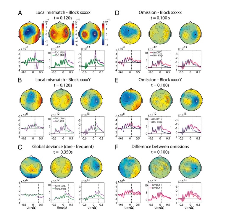
What we can see here is that local oddballs (first two plots on the left) and tone omissions (first two plots on the right) led to an early difference wave: in comparison with expected transitions, unexpected local changes and omissions elicit more neural activity very shortly after (anticipated) tone onset. This effect was evident in temporal and frontal sensors.
When it comes to global regularities, three interesting things happen. Firstly, a parietal sensor makes an appearance in addition to the temporal and frontal ones. Secondly, sensitivity to global regularities becomes visible later during tone processing compared to local transitions. It looks like local changes are early, while global changes are late. However, we can also look at the effects of local and global regularities in the absence of stimulation, when a tone is omitted. Contrary to the stimulus modulations by expectation, sensitivity to global regularities is here evident early – it emerges as early as the local difference wave.
Are the top-down effects of sensitivity to local and global regularities then concurrent, or not? This piqued my interest, so I kept on the lookout for papers that might tell me more.
Event-related potential, time-frequency, and functional connectivity facets of local and global auditory novelty processing: an intracranial study in humans.
El Karoui, I., King, J.R., Sitt, J., Meyniel, F., Van Gaal, S., Hasboun, D., Adam, C., Navarro, V., Baulac, M., Dehaene, S. Cohen, L., & Naccache, L. (2015). Cerebral Cortex, 25(11), 4203-4212. (link)
This is an ECoG study on 9 presurgical epileptic patients. The position of the electrodes provided temporal, frontal and parietal coverage.
- Block type 1: AAAAA is frequent among: AAAAA AAAAB
- Block type 2: AAAAB is frequent among: AAAAA AAAAB
Like in the previous study, the authors here compare local differences (when the final tone is a deviant vs. a standard), and global differences (when the final tone is expected vs. unexpected based on the block type).
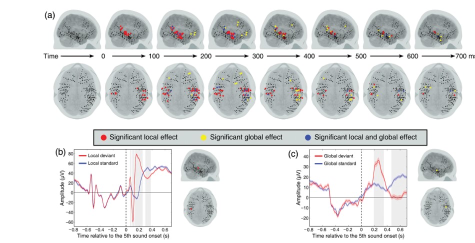
They looked for electrodes that show a difference in local as well as global expectation. They find these differences both in LFPs and in high gamma power. The local effect was evident about 100 ms earlier than the global effect. The local effect was restricted to temporal electrodes, whereas the global effect could be read off both temporal and frontal electrodes. Parietal areas don’t make an appearance. This left me to wonder whether the global effect evident in temporal areas get passed back down from frontal areas. The usual order of processing in the feedforward sweep would then be a good indicator of when a certain type prediction error would be resolved.
Hierarchy of prediction errors for auditory events in human temporal and frontal cortex.
Dürschmid, S., Edwards, E., Reichert, C., Dewar, C., Hinrichs, H., Heinze, H. J., Kirsch, H.E., Dalal, S.S., Deouell, L.Y., & Knight, R. T. (2016). Proceedings of the National Academy of Sciences, 201525030. (link)
This is also ECoG study, on 5 presurgical epileptic patients. The position of the electrodes again provided temporal, frontal and parietal coverage.
The stimuli were an unbroken train of tones, containing frequent standards and rare deviants. What differed per block was whether the deviants came at a predictable or unpredictable moment in time. In one block, the oddball was every fifth tone, while in the other block the distance between two oddballs varied. This means that the first type of block had a clear-cut global regularity to it, whereas the second one did not.
- Block type 1: AAAABAAAABAAAABAAAABAAAABAAAAB
- Block type 2: AAABAAAAAABAAABAAAABAAAABAAABA
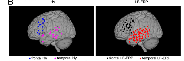
They first searched over the space of the sensors to see which ones were sensitive to the difference between the standards and oddballs (all As vs. all Bs). In order to have comparable sensitivity across different frequency bands (which carry different total power), they calculated an F-score per frequency, and looked then for clusters of electrodes using these scores. This allowed them to show that the difference in processing standards and oddballs is captured by LFPs and gamma power, but not the intermediate frequency bands.
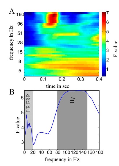
These differences were evident in temporal and frontal (but not parietal) sensors, with high gamma being present in fewer electrodes, but nearly always in those that also showed an LFP effect. The high gamma effect, to my surprise, preceded the LFP difference.
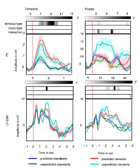
The crucial comparisons are whether block type – the presence vs. absence of a global regularity – will be evident in any of these electrodes (it wasn’t), and whether block type interacts with stimulus type (it does!). In the top right plot just above, frontal gamma decidedly increases with the temporally unpredictable oddballs very soon after stimulus onset – and while it stays low for all other combinations of stimulus and block. It’s as if the frontal cortex creates an error response only for deviations from global regularities. This error is not passed back down to temporal areas (which, at the same time, process the local difference between standards and oddballs, also in gamma), and does not become evident in the LFPs.
Take-home message
The best I can say is that it’s complicated. A number of small differences (in task, paradigm, sample, analysis pipeline) might be at the root of the differences in the results, but predictive coding models do not make clear predictions on what these differences should be. Small samples too, which is common for technically complex studies.
Where in the brain? Temporal and frontal areas continue to come through as crucial to mismatch negativity. A variety of subcortical auditory areas (e.g. the inferior colliculus or medial geniculate body), are not picked up by the types of imaging used here, but could in principle also be involved. Some of the results point to local mismatches being processed in temporal areas and global mismatches in frontal, but some of the results show that this separation is not absolute and that the mismatches might be passed both up and down.
When in the brain? Some of these results point to local and global mismatches being processed one after the other, others point to concurrent processing.
What type of neural activity? Low frequencies (probably capturing the energy of the evoked response) and high gamma (probably multi-unit activity) – but it is unclear if one drives the other. If gamma is feedforward error signalling, where is the frontal gamma feeding forward to? Changes in alpha/beta power, so common in the predictive coding literature, don’t make an appearance. I would guess that they are a better marker for visual processing, and that their generality gets overstated.
Does this resolve some issues about predictive coding works? Or does it add to them? What are your open questions about predictive coding? I’d love to hear them, to add to my growing confusion.